Reconstructing Column Data from .idf and .idfmeta

If metadata.sqlitedb tells you what the model means and .dictionary tells you what the IDs mean, .idf and .idfmeta tell you how the payload itself is packed on disk.

This is the layer where a PBIX parser either becomes a real data extractor or stays a metadata browser.

Where This Fits

This is the lowest-level storage article in the launch batch. It builds directly on The DataModel article and VertiPaq Dictionaries and Hash Indexes. If you only want the high-level API, skip to Parsing PBIX Files with Python (pbixray).

What the Two Files Do

For each stored column segment, VertiPaq separates metadata from payload:

• .idfmeta describes how the segment is encoded
• .idf stores the encoded values

That split is crucial. You cannot decode the .idf bytes correctly by looking at them in isolation. You need the companion metadata to know where RLE applies, where bit-packed values begin, and how to interpret the resulting integers.

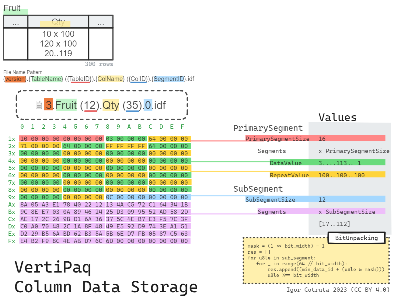
The Shape of .idf

Structurally an .idf file is a sequence of segments, each built from a variable-length primary segment followed by a variable-length sub-segment:

segment:
  seq:
    - id: primary_segment_size
      type: u8
    - id: primary_segment
      type: segment_entry
      repeat: expr
      repeat-expr: primary_segment_size
    - id: sub_segment_size
      type: u8
    - id: sub_segment
      type: u8
      repeat: expr
      repeat-expr: sub_segment_size

segment_entry:
  seq:
    - id: data_value
      type: u4
    - id: repeat_value
      type: u4

Each primary-segment entry is just two u4 fields: data_value and repeat_value. That already hints at the hybrid strategy. Most entries behave as straight RLE runs. A special marker (data_value == 0xFFFFFFFF) indicates that the next repeat_value records must be read from the bit-packed sub-segment instead.

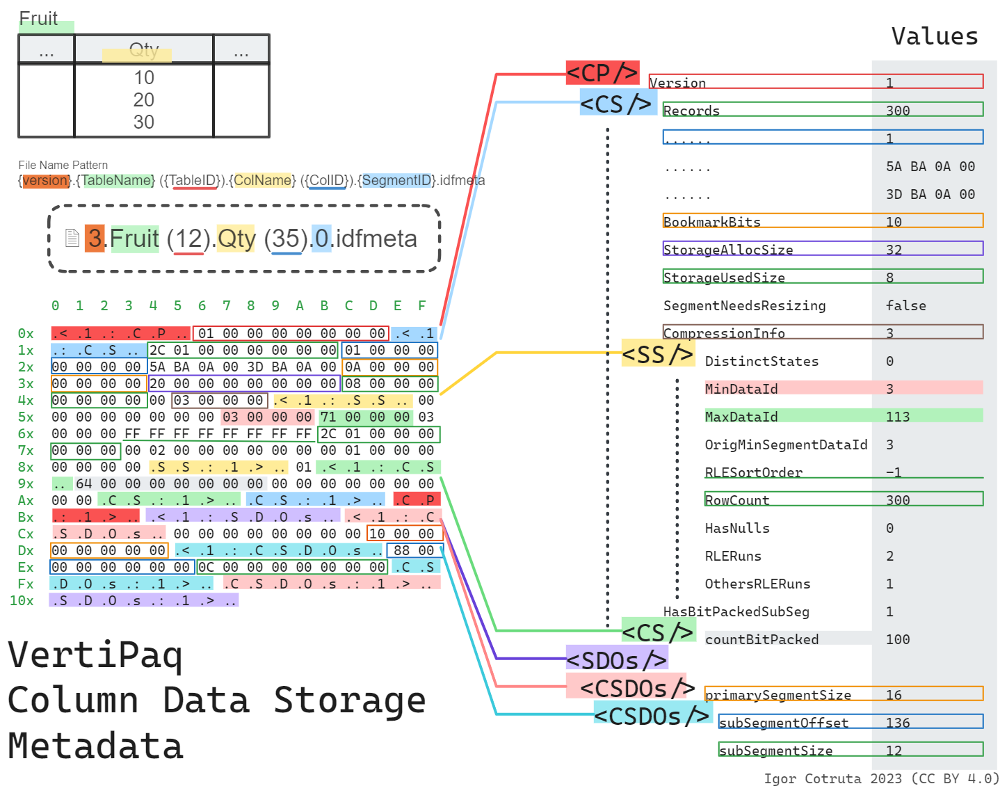
The Shape of .idfmeta

The .idfmeta companion is much richer. It uses a tagged binary format where every block is wrapped in textual markers — <1:CP\0 opens a column partition and CP:1>\0 closes it, with <1:CS\0/CS:1>\0 for each column segment and <1:SS\0/SS:1>\0 for the subsegment statistics nested inside. You can often pick an .idfmeta file out of a hex dump just by spotting those tags.

Inside that envelope lives a compression_class identifier (a PF_OBJECT_CLASS value) that tells the decoder exactly how the segment is encoded:

• 0x000aba37–0x000aba40, 0x000aba42, 0x000aba46, 0x000aba4b, 0x000aba56 are fixed-width bit-packing for 1–10, 12, 16, 21, and 32 bits respectively
• 0x000aba5a is the common Hybrid RLE form — this is where the .idfmeta also carries a sub_compression_class (one of the fixed-width IDs above) that says how the bit-packed sub-segment is encoded
• 0x000aba57 is general compression (no fixed bit width), 0x000aba5b is a 123-style variant

For table reconstruction, a parser typically only needs a small subset of the available metadata:

• minimum data ID
• bit width (derived from compression_class or sub_compression_class)
• count of bit-packed values
• compression-related segment metadata

The current pbixray decoder extracts exactly those essentials:

row_data = {
    "min_data_id": metadata.blocks.cp.cs.ss.min_data_id,
    "count_bit_packed": metadata.blocks.cp.cs.cs.count_bit_packed,
    "bit_width": metadata.bit_width,
}

Hybrid RLE plus Bit Packing

The storage strategy described by the two files is hybrid:

• use RLE where long runs exist
• use tightly bit-packed integers where the data is more heterogeneous

In the pbixray implementation, the primary segment is walked entry by entry. Ordinary entries expand to repeated values. A special marker value means “switch to the next batch of bit-packed values from the sub-segment.”

Conceptually it looks like this:

primary segment:
  [value, count]
  [value, count]
  [0xFFFFFFFF, count]   -- marker: next `count` entries come from sub-segment

sub-segment:
  packed integers with width = bit_width

The pbixray decoder tracks a rolling bit_packed_offset so that successive bit-pack markers pull the next batch of values out of the sub-segment correctly — the marker is detected by checking entry.data_value + bit_packed_offset == 0xFFFFFFFF, then the offset advances by entry.repeat_value.

That design lets VertiPaq take advantage of both repetition and compact integer widths within the same column segment.

min_data_id, bit_width, and the Reconstructed Vector

Once the parser knows the bit width and the minimum data ID, it can unpack the sub-segment into actual integer values. In pbixray, each 64-bit word is shifted and masked repeatedly:

mask = (1 << bit_width) - 1
res.append(min_data_id + (u8le & mask))
u8le >>= bit_width

Those integers are still not final business values. They are the reconstructed encoded vector. That vector then flows into:

• dictionary mapping for dictionary-backed columns
• BaseId and Magnitude scaling for value-encoded numerics

The End-to-End Column Reconstruction Flow

Putting the pieces together, a direct parser usually follows this sequence for each stored column:

1. use metadata.sqlitedb to locate the relevant files and column properties
2. parse .idfmeta to get min_data_id, count_bit_packed, and bit_width
3. parse .idf to rebuild the encoded vector from RLE and bit-packed segments
4. map the encoded vector through the dictionary path or the value-encoding path
5. cast the result to the final runtime type

That five-step flow is the heart of imported-table reconstruction in pbixray.

Why This Is the Hardest Part of the Format

This layer is where multiple incomplete truths have to line up:

• the segment payload alone is not enough
• the metadata alone is not enough
• the dictionary alone is not enough

Only when all three agree do you get a faithful column back out. That is why so much of the reverse-engineering effort ends up concentrated here.

Related Articles

• Read Inside metadata.sqlitedb: Tables, Columns, Measures & Relationships for the metadata that points to these files.
• Read VertiPaq Dictionaries and Hash Indexes for the final value-mapping stage.
• Read How VertiPaq Sorts Rows to Maximize RLE Compression for why the choice of row order can move Hybrid RLE efficiency by an order of magnitude.
• Read Parsing PBIX Files with Python (pbixray) for the API that hides this complexity behind get_table().